Tidy text analysis of the leaked Trump phone calls

Last week I read the leaked phone calls between Donald Trump, and the leaders of Mexico, and Australia, and I was again shocked a bit, by the president’s command of the English language. Coincidently, I wanted to read, and try out the things in the Tidy Textmining in R book, so here we are.

if (!require("pacman")) install.packages("pacman")
pacman::p_load(rprojroot,
               tidyverse,
               ggplot2,
               dplyr,
               rvest,
               stringi,
               tidytext,
               knitr)

# setting project root, and creating temp folder for images
# root <- find_root(is_rstudio_project)

For start I downloaded the text for both conversations seperately. The Washington Post’s developers created a pretty great structure for the transcript’s site. Everything is neatly nested hiearhically. For example there is a mexico class, which has a transcript, and transcript-container class in it, and inside them there is a seperate class for the different leaders.
I used the rvest package to download the text from the site. As you can see from the code, getting the required parts of the text was pretty straight forward, and thanks to the site’s structure, the code is pretty expressive.
I downloaded only Trump’s sentences, and I downloaded them seperately for both calls. I created an unary function, because I wanted to apply the same transformations on both text, but didn’t want to repeat code.

transcripts <- read_html("https://www.washingtonpost.com/graphics/2017/politics/australia-mexico-transcripts/")

mexico <- transcripts %>%
  html_nodes(".mexico .trump p") %>%
  html_text()

australia <- transcripts %>%
  html_nodes(".australia .trump p") %>%
  html_text()

clean <- . %>%
<<<<<<< HEAD
  data.frame(sentences = ., stringsAsFactors = FALSE) %>%
=======
  data_frame(line = 1:length(.), sentences = .) %>%
  # unnest_tokens does conv to lowercase, punctuation removal
>>>>>>> 562d7699657fba1936ad94b57acaeef8690e5b11
  unnest_tokens(word, sentences) %>%
  anti_join(by = "word", stop_words)

I also created a new column, which shows which sentence belongs to which call. After this I joined the two conversations back together.
Maybe one could do the above thing more elegantly, for example use apply and NSE in a creative way (i.e. create a list with the country names, use apply on them and the pipe sequence, and pass them to the new column). I might do this in the future, if it’s feasible.

mexico_words <- mexico %>% clean %>% mutate(call = "Mexico")
australia_words <- australia %>% clean %>% mutate(call = "Australia")

word_counts <- rbind(mexico_words,
                     australia_words)

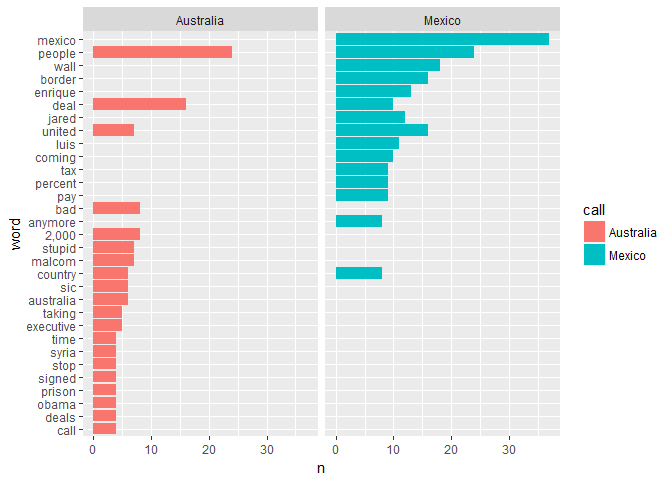
Next, I filtered out the 15 most used words by Trump, and created a bar chart for them:

word_counts %>%
  group_by(call) %>%
  count(word, sort = TRUE) %>%
  top_n(15, n) %>%
  ungroup() %>%
  mutate(word = reorder(word, n)) %>%
  ggplot(aes(x = word, y = n, fill = call)) +
  geom_col() +
  coord_flip() +
  facet_wrap(~ call)