Recreating Washing Post's solar eclipse plot in R
I will continue copycatting visualization in this post.
This I seen the following visualization from a couple of difference sources:
Oh, this is cool. https://t.co/eCSKI6ag3P pic.twitter.com/BoBlMjZGV7
— Teddy Amenabar (@TeddyAmen) July 10, 2017
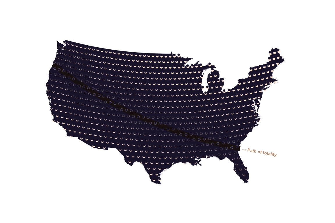
I thought this would also be a good vis to recreate. I had a couple of different ideas on how to recreate it, but little did I know how difficult it would be. Disclaimer: I created this purely with geometrically, it doesn’t represent the true path of of an eclipse.
if (!require("pacman")) install.packages("pacman")
pacman::p_load(rprojroot,
               tidyverse,
               purrr,
               splancs,
               data.table,
               knitr)

# setting project root, and creating temp folder for images
root <- find_root(is_rstudio_project)

opts_knit$set(root.dir = root)

img_tmp <- "/tmp/img/"
dir.create(paste0(root, img_tmp), recursive = TRUE)

# eclipse line parameters
line_int <- 7
line_slope <- -0.3

# min-max of the longitudes and latitudes for the map
long_min <- -125
long_max <- -67
lat_min <- 25.75
lat_max <- 49

# parameters for the eclipse grid
long_pack <- 1.1
lat_pack <- long_pack * 0.9

# creating eclipse grid
long_coords <- seq(from = long_min, to = long_max, by = long_pack)
lat_coords <- seq(from = lat_min, to = lat_max, by = lat_pack)
points <- data.table(CJ(long = long_coords, lat = lat_coords))

# shifting every even row horizontally
long_to_shift <- seq(from = lat_min, to = lat_max, by = lat_pack * 2)
points[points$lat %in% long_to_shift, long := long + (long_pack/2)]
The basics of the visualization seems pretty easy, you creates eclipses with differnt occlusions on a grid. First I thougth it would be difficult to do this properly, so I wanted to use emojis or unicode for it. Alas I couldn’t plot the special characters on the plot, which was ultimatelly fortunate, because the next day I had an idea for a real neat sollution. I plot two point in a grid point, one for the sun, on for the moon, and I offset one by a given number. For this offset I used the distance from the eclipse line, which I calculated below with the function borrowed from [stackoverflow][dist_fun]. I scale this distance to a range, which I can multiple up later so that it fits with the plotted point’s size.
# from: https://stackoverflow.com/questions/35194048/using-r-how-to-calculate-the-distance-from-one-point-to-a-line
dist2d <- function(a,b,c) {
  v1 <- c - b
  v2 <- b - a
  m <- cbind(v1,v2)
  d <- abs(det(m))/sqrt(sum(v1*v1))
}

line_left <- c(long_min, long_min * line_slope + line_int)
line_right <- c(long_max, long_max * line_slope + line_int)

# map from: http://eriqande.github.io/rep-res-web/lectures/making-maps-with-r.html
usa <- map_data("usa")

# keep only grid point that are inside the country
# from: https://stackoverflow.com/questions/17571602/r-filter-coordinates
points <- points[inpip(points[,c("long", "lat")], usa[,c("long","lat")]),]

# calcualting distance from the eclipse line for every grid point
points$dist <- map2_dbl(.x = points$long, .y = points$lat,
                        ~ dist2d(c(.x, .y), line_left, line_right))

# scale point distance to [0,1]
# from: https://stackoverflow.com/questions/5468280/scale-a-series-between-two-points/5468527#5468527
scaled <- function(x) {
  (x - min(x)) / (max(x) - min(x))
}
points$dist_scaled <- scaled(points$dist)
Two tricks I had to use were the following, first I had to filter the point that are inside of the map, and secondly in the original plot the eclipses “below” the eclipse line deviated in a differnt directiont that those that are “above” it. For this I created two filters. For both I used the inpip function from the splancs package. This filters points by looking if there are inside a polygon or not. First I filtered with the US map polygon, and in the second filter I created a polygon that encompases the area above the line. This was a pretty elegant sollution in the end, because at first I wanted to implement it with a signed distance function.
# lower triangle for point that are "under" the line
upper_poly <- data.table(x = c(long_min, long_min, long_max, long_max),
                         y = c(lat_max, line_left[2], line_right[2], lat_max))

points[inpip(points[,c("long", "lat")], upper_poly),
       dist_scaled := dist_scaled * -1]

# create eclipse line manually
ecl_l <- -124
ecl_r <- -81
ecl_line <- data.table(x = c(ecl_l,
                             ecl_r),
                       y = c(ecl_l * line_slope + line_int,
                             ecl_r * line_slope + line_int))
Finally I plotted the result:
# plot params
bias <- 0.35
point_size <- long_pack * 2

eclipse <- ggplot() +
  # US map
  geom_polygon(data = usa, aes(x=long, y = lat, group = group),
               fill = "#221a38") +
  coord_fixed(1.2) +
  # manual eclipse line
  geom_path(data = ecl_line, aes(x = x , y = y), color = "#201216", size = 6) +
  # sun halo
  geom_point(data = points, aes(x = long, y = lat), size = point_size*1.15,
             alpha = 0.2, color = "#ffebdb") +
  geom_point(data = points, aes(x = long, y = lat), size = point_size*1.3,
             alpha = 0.1, color = "#ffebdb") +
  # sun
  geom_point(data = points, aes(x = long, y = lat),
             size = point_size, color = "#ffebdb") +
  # moon
  geom_point(data = points, aes(x = long,
                                y = lat + bias * dist_scaled),
             size = point_size,  color = "#221a38") +
  # eclipse line annotation
  annotate("text", x = ecl_line[2,1] + 3.8, y = ecl_line[2,2] - 1.1,
           label = "\u2192 Path of totality",
           color = "#C0977A", fontface = 2, angle = -10) +
  coord_map("albers", lat0=30, lat1=40) +
  # from: https://stackoverflow.com/questions/14313285/ggplot2-theme-with-no-axes-or-grid
  theme(line = element_blank(),
        text = element_blank(),
        title = element_blank(),
        panel.background = element_blank())

eclipse
# I save it to png first so ggplot2 renders it the same on all of my computers
# ggsave(paste0(root, img_tmp, "eclipse.png"), eclipse,
#        width = 12, height = 8)
# knitr::include_graphics(paste0(root, img_tmp, "eclipse.png"))